Here you can download some of best games that can be played in Excel. Just download it and start playing in your excel :)
 Adrenaline Challenge:This is a motor cycle game with predefined objectives. Complete the objectives as fast as possible and move to the next stage.
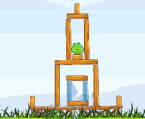 Angry Birds: I can bet that most of us would have played angry birds before, but this is a handy flash version of the game. This is a must try for all the angry birds lovers.
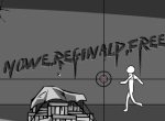 Bang Bang -2: Bang Bang-2 is a first person shooting game. Your objective is to kill as many people in the stipulated time.
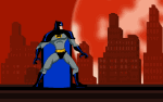 Batman: Play the heroic Batman game to save the Gotham city from bad people. Defeat the bad people and move to the next levels.
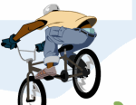 BMX-Tricks: Ride your cycle and perform different stunts on the track to earn extra points in stipulated time. You can ride over grills, on tables etc. to earn extra points.
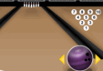 Bowling: This is a cool game with 3D graphics. Aim the bowl using the mouse to hit the pins. A must try game for bowling lovers.
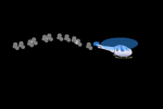 Chopper Challenge: Fly the chopper as far as possible and avoid the obstacles in the path. Make a high score and challenge your friends.
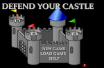 Defend Your Castle: Defend Your Castle was one of the most rated games of 2012. Here your goal is to protect your castle from the opponent team.
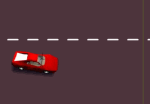 Drunk Driving: In this game your task is to handle an uncontrollable car. Avoid the obstacles like other cars and buses to clear stages.
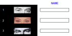 Famous Eyes: This game consists of images of eyes of some of the famous personalities, identify them and earn points.
 Frog leap: This is a little puzzle game. The game challenges you to interchange the positions of 6 frogs. Clear the level and challenge your friends.
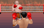
2D Knockout: 2D knockout is a boxing game. You have to play against the boxers of various countries. The objective of this game is to defeat your opponent.
Download it here.
3D Tic Tac Toe:3D Tic Tac Toe is a must try game for all the tic tac toe lovers. The objective of the game is to get 4 X’s or 0’s in a row, whosoever gets it first wins the game.
You can download this game here.
Adrenaline Challenge:This is a motor cycle game with predefined objectives. Complete the objectives as fast as possible and move to the next stage.
Get it here.
Air Fighting: This is a traditional Air Plane fighting game. The objective of this game is to destroy all the opponent air planes.
Click this link to download.
Angry Birds: I can bet that most of us would have played angry birds before, but this is a handy flash version of the game. This is a must try for all the angry birds lovers.
You can download this game here.
Angry birds Rio: This is another angry bird’s game with bigger and better graphics. I am quite sure that you will fell in love with this one.
Download it here.
Apple Shooter: Apple shooter is a very nice game designed by Wolf games. Here your objective is to shoot the apple without killing the man beneath it.
Get it here.
Ball Challenge: This game has a set of blue and red balls bouncing inside a box. You need to keep the blue balls inside one compartment and the red ones inside another compartment.
Click this link to download.
Bang Bang -2: Bang Bang-2 is a first person shooting game. Your objective is to kill as many people in the stipulated time.
Excel game here.
Baseball Pinch Hitter -2: This game has awesome graphics and great gameplay. The game has certain levels and you have to meet some targets to clear those level.
You can download this game here.
Batman: Play the heroic Batman game to save the Gotham city from bad people. Defeat the bad people and move to the next levels.
Download it here.
Bloxorz: The aim of this game is to roll the block such that it falls in the square hole inside the board. The game has 33 stages and different challenges that you will love to tackle.
Get it here.
BMX-Tricks: Ride your cycle and perform different stunts on the track to earn extra points in stipulated time. You can ride over grills, on tables etc. to earn extra points.
Click this link to download.
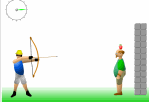
BowMan: This is a third person shooting game where you have to kill your opponent using arrows. You can shoot the arrow at different angles and power to hit the opponent.
You can download this game here.
Bowling: This is a cool game with 3D graphics. Aim the bowl using the mouse to hit the pins. A must try game for bowling lovers.
Download it here.
Chaser: This is a nice time pass game. The game is very similar to the traditional snake’s game with the only difference that you and computer are playing on the same board.
Get it here.
Chopper Challenge: Fly the chopper as far as possible and avoid the obstacles in the path. Make a high score and challenge your friends.
Click this link to download.
Crab Ball: This a little funny volleyball like game between two crabs. Simply download the game and enjoy playing it.
Excel game here.
Defend Your Castle: Defend Your Castle was one of the most rated games of 2012. Here your goal is to protect your castle from the opponent team.
Download the game here.
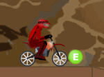
Down Hill Stunts: This is a motor bike game, your aim is to ride your bike on the track and collect the stars on the way and that too without crashing.
Download it here.
Drunk Driving: In this game your task is to handle an uncontrollable car. Avoid the obstacles like other cars and buses to clear stages.
You can download this game here.
Easy Chess: This a flash version of the chess game. A must try game for a die-hard chess lover.
Download it here.
Famous Eyes: This game consists of images of eyes of some of the famous personalities, identify them and earn points.
Get it here.
Fishy: Fishy is small time pass game, where you have to feed your fish on the other small fishes and also save your fish from the other fishes that are bigger than it.
Click this link to download.
Frog leap: This is a little puzzle game. The game challenges you to interchange the positions of 6 frogs. Clear the level and challenge your friends.
Excel game here.
Golf: The main objective of this game is to put the ball inside the hole in minimum number of strokes. The game also offers a multiplayer mode.
Download the game here.