Windows 10 is the latest version of Windows Operating System and so far it's good.Windows 10 is a free upgrade for Windows 7, Windows 8, and Windows 8.1 users, but those running older versions may have to buy a copy. But if want to Activate your Windows 10 for free you can use Windows 10 Activation Key and Serial Key that are provided on Technoration.
The VLOOKUP is one of the most used formulas in Excel across all sorts of different industries. The “V” in VLOOKUP stands for vertical. It allows you to compare two lists. The formula looks for a value in the left most column of a worksheet of data and if it finds that value it returns the value from the same row in a column specified by you. This is a big one and an important formula so it gets its own tab on the companion Excel workbook. Formula: VLOOKUP(lookup_value,table_array,col_index_num,range_lookup)
Let’s take a look at the anatomy of a VLOOKUP:
The “lookup_value” is the value you are looking for, to see if it is in both lists. The “table_array” is the table that you are going to have the formula look in. This is just a reference to the cells you want to look in. The “Col_Index_Num” is the column number you want the formula to return if it finds a match. The “Col_Index_Num” is the column you want to be returned if there is a match. It is relative to the first column which is 1. If you start in column A and you want to return whatever is in column C you would put a 3 in the column. The “Range_Lookup” is a “TRUE” or “FALSE” argument that tells Excel whether you want an exact match or a partial match. I’ve personally never used anything but an exact match, which is the “FALSE” argument.
The Example on the workbook
The example on the workbook compares two lists. One list has a list of trader names and the trader’s ID number. The other list has the stock name and the trader’s ID number. Our objective is to compare the first list to the second list and match the trader name to the stock on the second list. We do this using the formula: =VLOOKUP(F11, $A$10:$B$33, 2, FALSE).
Our Data lists for the VLOOKUP example
Let’s break it down:
The “lookup_value” in our formula is F11 for the first row of the formula (Remember this is a relative reference because there are no $, so this cell reference will change when we drag the cell in down). Cell F11 is the ID number on the second list. The ID number is our unique identifier.
The unique identifier has to be the same on both lists that you are comparing. Numbers are usually best, but it can be text. This is what you use to compare the two lists. In our example we use the trader’s ID number as our unique identifier because it is on both lists and there is only one ID number for each trader on the list, making it unique. The “table_array” is the area that you want Excel to look in to compare the two lists. In our example we we excel to look in the range “$A$10:$B$33”. It will look in the first column in the “table_array” for the “lookup_value”. The “col_index_number” is the column number you want returned, relative to the first column in the “table_array”. Let’s use our example to understand this. The first column in our “table_array” is column A, this is column number 1. When the VLOOKUP finds a match we want the data next to it to be the return value, so we put “2” as our “col_index_number” because we want the value in the 2nd column of our “table_array” returned whenever there is a match. The “range_lookup” value is the true or false argument saying whether you want the “lookup_value” to be an exact match or a partial match. We used “FALSE” because it has to be an exact match in order for it to be returned.
In our example it is looking for the value of cell F11 in the range “$A$10:$A$33”. If it finds a match it will return what is next to that cell in the range “$B$10:$B$33”, because the “col_index_number” is 2. In our example cell F11’s value is 15. The VLOOKUP looks for 15 in the range “$A$10:$B$33” it finds a match in cell A25 and it returns what is in cell B25, the trader’s name: Mike. We then drag this formula down the entire list and we easily get the trader name matched to a the stock they are responsible for.
Did you know that you can create multiple email addresses with one Gmail address . Yes it is possible and not most of us are aware of the few tricks involved to achieve this. You may ask why would you need multiple email addresses for your Gmail address? Let me explain it to you.
The point here is to make multiple email address from your primary Gmail address and create unique email addresses for registering with different websites and services. In fact you can have many different email addresses for your primary Gmail address, but all the mails send to these secondary email addresses will be received in your primary Gmail addresses inbox.
This way you can create a filter for each of the custom email address associated with your Gmail account and easily organize emails from different services and websites. If in any case a website starts sending spam into your inbox , you can easily set the specific filter in your Gmail account to delete all the mails instantly when received in your inbox.
Now lets find out how we can create multiple email addresses from your Gmail address. There are two methods for creating multiple email addresses for your Gmail address.
Method 1: Using “+” annotation in your Gmail address
If you want to create multiple email addresses from your Gmail address then you can use the “+” symbol to add another word to your Gmail address. For example,
Suppose your Gmail address is peterparker@Gmail.com and you want to create a custom email address for signing with amazon.com . To create this custom email address , all you need to do is just add the keyword “amazon “ before or after your username in your email address like this “ peterparker+amazon@Gmail.com” or “amazon+peterparker@gmail.com” and sign up with it on Amazon.com. Now all the emails from both these emails will be sent to your primary Gmail address at peterparker@Gmail.com .
It is as simple as that and you can use this simple trick to create an unlimited number of custom email addresses and all of the mails would be send to your primary Gmail address .
Method 2: Using dots in your Gmail address
Coming to the second method, its an less known fact about Gmail. Gmail does not care about how many dots you have in your email address. In fact it doesn’t recognize any dots within a Gmail address, which means you can place any number of dots within your Gmail address before the @ tag and Gmail will ignore the dots and still send the mail to your original mail address sans the dots. For example ,
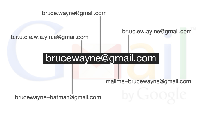
Lets take your email address to be brucewayne@Gmail.com . If you add a dot anywhere within the words “brucewayne” , Gmail will always ignore the dots. Example you can create multiple emails address like the below :
bruce.wayne@Gmail.com
br.uc.ew.ay.ne@Gmail.com
bruce.way.ne@Gmail.com
b.r.u.c.e.w.a.y.n.e@Gmail.com and a lot more .
All these above Gmail address will still point towards your primary Gmail address at brucewayne@Gmail.com . Depending upon your requirement you can have many uses of these tricks , even you can use these tricks to update your Gmail address . Go ahead and try create as many custom email address as you would like for your Gmail address . and do let us know how this was useful to you . Keep subscribed for us to know about more interesting how to tips and tricks .
There are very less antivirus software companies that have made their name in security applications, Panda Security is one of the few. All of its products are great for home as well as office use. Panda Internet Security 2015 provides many features other than security, which are beneficial to any home user. Online backup, parental control, and data shield are some of the features of Panda Internet Security 2015, in addition to protecting your system from viruses and malware at all times.
There are often situations when you need to track the location of the person you’re talking to. Not always, but sometimes its really urgent. So, we have come here with three best methods to help you be aware :
1. Through Facebook Chat
This is fast,but a little tricky as well, thought its pretty straight forward. Many people have used this method and its been a success. You need to be friends with whoever you want to track on Facebook. Next have a conversation with that friend on Facebook. Make sure all other tabs remain closed, and no application is running on the background that consumes your net.
Next, follow these :
Press Win+R , a shortcut it us.
Next you type cmd and enter.
In the command prompt that appears, type netstat -an and click enter.
This now provides to you with a list of IP addresses, which will have the person’s address whom you are chatting too as well.
You now have to have a look at the possible IP of the person.
Next you have to go tohttp://www.ip-adress.com/ip_tracer/ and then type the IP address on the box which says “lookup this ip or website”
And there you go!
2. By Creating Tracking Link
this is a better source than the first one. Also, once done, it lets you track the addresses.Basically you are to great a link which will save their IP address with timestamp and user-agent/browser.
All you do is follow as stated below:
Visit a website such as 000webhost, ByteHost, Free Hostia, etc. (See Full List of Free Web Hosting Sites Here)
Now you need to make up a domain name and register yourself there for free. May be a sub domain such yoursite.freehosting.com. And aslo make sure you can add up your own files..
Next you have to download a zip file: Track-IP
You will see files, Namely: img.jpg, index.php and log.txt. You need to out them up on your free website root.
Now, the link you created, (yoursite.freehosting.com), this will be your tracking link. You send it to the person, and make sure that they visit it
Once they click on the URL, the log.txt file will trace their IP, Browser along with the timestamp. And now you are through!*This works out better on email*
3. Using Website Tracing Scripts
This needs you to have a website.
Now the steps:
Add the Google Analytics tracking code on your website.
Create a link of your website. A dummy post would be more preferable.
Just like in the above method you need to make them click over the link you just sent.
If you happen to be online, you would be able to see them on your Google Analytics account for the link. Otherwise you cab visit their later, and check out the history and other details.
For the user’s stat, Google Analytics is a lot more derailed.
There are other tracking links such as Histats, Statcounter, etc.
Excel provides an enormous number of established formulas and assistance in auditing and calculating your data. The primary groupings are financial, logical, text, date and time, lookup and reference, math and trigonometry, statistical, engineering, cube, and file-related information.
How many times you created a chart in Microsoft excel and formatted it for minutes (and sometimes hours) to reduce the eye-sore?
Well, I will tell you my answer, its 293049430493 times
Worry not! for you can become a charting superman (or elastigirl) by using these 73 free designer quality chart templates in literally no time (well, almost)
Microsoft Excel is the most useful and easy tool for business analysts. It has large number of useful formulas, features and bundles of interactive charts. But, most of us are not known of all of them and there are some more features which are powerful and easy to use to make our work simpler. You might not have noticed some of the useful Excel 2010 & 2013 features like Sparklines, Slicers, Conditional Formatting and other formulas which add value to your work. In this article, I will take you through them and will give you an idea on what are those and how to use them.
Most Useful Excel Features
Among many Excel features, there are some hidden features which are easy to use and you many not know all of them. Without any further delay, we will look at 5 such Excel features.
Sparklines
Sparklines were first introduced in Excel 2010 and are used to represent visualizations for the trend across the data in a row. It fits in a single Excel cell and saves the space on the worksheet. This is a cool feature and is very easy to use. Calculating the trend for row data and placing the visualization in the single excel is really a great feature to use.
In order to create your own Sparklines, select the range of data. Click insert on the ribbon and select the type of Sparklines (Line, Column or Win/Loss). Next, enter the range of the target where you want to show the Sparklines.
Conditional Formatting
Conditional Formatting is a well known feature of Excel. It is used to visually present the data based on the conditions met. It is also useful to create heat maps. This would be helpful to find the interesting patterns by exploring the data effectively.
To create the heat map, select the data and head over to the ribbon. Under Home, clickConditional Formatting and then click Color Scales. Now, pick the color scale. You can even set the color scale by editing the formatting rule.
SMALL and LARGE Functions
We all know about MAX and MIN functions. They give you the maximum and minimum values of the selected data respectively. But, in order to find the 1st, 2nd, 3rd or nth largest or smallest value of the selected range if data, we can make use of LARGE and SMALL functions respectively.
In this example, in order to find the top two products for each month, we made use of MATCH and INDEX functions along with LARGE and SMALL functions.
Remove Duplicates
Do not blame me for mentioning this feature in this list. It is very important to get rid of redundant data from the available huge amount of data. It is one of the best ways for cleaning and organizing the data and so thought of having it in this list of powerful Excel features. Removing Duplicates feature was introduced from Excel 2007 and is helpful to remove duplicates which is the most important problem which we face.
To remove duplicates, select the data and head over to the ribbon. Under Data, click theRemove Duplicates button and what you see the data without duplicates.
Slicers
Slicers act as visual filters. It helps you to visualize the subset of data as a connected chart or as a raw data. For example, if you want to show the trend of sales of various products, then you can create the interactive sales trend chart using Slicers. Based on the product you select, respective chart is shown. Slicers were first introduced in Excel 2010 and enhanced a lot in Excel 2013.
In Excel 2013, if you want to add Slicer to your charts, select the data range and click on insert > Slicer. Now, select the part of the data you want to use as a filter. In the image above, Product column is used as a filter.
How many of you have used these powerful and useful Excel features? If you want to add more features to the list, please let us know through comments.
People often ask about the best principles to follow to make the better excel spreadsheets. Hope you might also be interested to know them. Here we go…
In the activity you will create and interactive game for elementary kids. There will be 9 questions and if the student answers them correctly it will reveal a picture underneath. The picture we will use for this activity is the shown below. Save it to your student folder.
Open Microsoft Excel 2007: Start > All Programs > Microsoft Office > Microsoft Excel 2007
Making a budget is pretty simple. But before I outline how to make a budget, I need to explain what I believe is the number one key concept in budgeting: A Budget is a Plan. "Budgeting" and "Planning" are synonymous.
"A budget is a plan for how you are going to spend your money"
A popular cliche applies here: "If You Fail to Plan, You Plan to Fail". When you break your budget, you are messing up your plan. When you stick to a budget, you are sticking to a plan. Which one sounds more optimistic?
A budget is often hated because people are always fighting against their budget. So what I want you to do when you make a budget is think of it and talk about it as a plan. Make a plan for how to spend your money and stick to your plan. I think this new point of view will help you be more optimistic, and it is certainly more empowering.
I’ve always believed that Excel is one of the most powerful software tools out there. It isn’t just the fact that it’s spreadsheet software, which is by its nature powerful anyway.
No, Microsoft Excel 2013 itself has such an awesome collection of built-in tools and features that it has beyond any doubt, become one of the most useful tools for so many things. In this article, I plan to show you how powerful formulas and conditional formatting can be, with three pretty useful examples.
Chapter III: Multiple Sets of Data in a Single Graph
Description :Download free Making Graphs In Microsoft Excel 2013: A Short Tutorial course material, tutorial training, PDF file by Justin Feng on 19 pages.
Microsoft Excel is program designed to efficiently manage spreadsheets and analyze
data. It contains both basic and advanced features that anyone can learn. Once some
basic features are known, learning the advanced tools becomes easy. This lesson is
composed of some advanced Excel features.
. It assumes basic prior knowledge of Excel, and it is expected that the objectives from AT Step’s Excel Essentials are known. This lesson will talk about the advanced customization and formatting features that allow for easier data manipulation and organization.
Objectives
1) Learn how to Customize the Interface
2) Advanced Formatting: Custom Lists, Cell Groups, and Transposing Tables
3) Learn how to Reference Across Sheets
4) Advanced Formulas and Using Data Ranges
5) Using Data Validation
Microsoft Excel is the most useful and easy tool for business analysts. It has large number of useful formulas, features and bundles of interactive charts. But, most of us are not known of all of them and there are some more features which are powerful and easy to use to make our work simpler. You might not have noticed some of the useful Excel 2010 & 2013 features like Sparklines, Slicers, Conditional Formatting and other formulas which add value to your work. In this article, I will take you through them and will give you an idea on what are those and how to use them.
Most Useful Excel Features
Among many Excel features, there are some hidden features which are easy to use and you many not know all of them. Without any further delay, we will look at 5 such Excel features.
Sparklines
Sparklines were first introduced in Excel 2010 and are used to represent visualizations for the trend across the data in a row. It fits in a single Excel cell and saves the space on the worksheet. This is a cool feature and is very easy to use. Calculating the trend for row data and placing the visualization in the single excel is really a great feature to use.
In order to create your own Sparklines, select the range of data. Click insert on the ribbon and select the type of Sparklines (Line, Column or Win/Loss). Next, enter the range of the target where you want to show the Sparklines.For more information on how to create neat charts & graphs in excel click here
Conditional Formatting
Conditional Formatting is a well known feature of Excel. It is used to visually present the data based on the conditions met. It is also useful to create heat maps. This would be helpful to find the interesting patterns by exploring the data effectively.
To create the heat map, select the data and head over to the ribbon. Under Home, clickConditional Formatting and then click Color Scales. Now, pick the color scale. You can even set the color scale by editing the formatting rule.
SMALL and LARGE Functions
We all know about MAX and MIN functions. They give you the maximum and minimum values of the selected data respectively. But, in order to find the 1st, 2nd, 3rd or nth largest or smallest value of the selected range if data, we can make use of LARGE and SMALL functions respectively.
In this example, in order to find the top two products for each month, we made use of MATCH and INDEX functions along with LARGE and SMALL functions. For more information on basic to advanced Excel formulas, visit this tutorial
Remove Duplicates
Do not blame me for mentioning this feature in this list. It is very important to get rid of redundant data from the available huge amount of data. It is one of the best ways for cleaning and organizing the data and so thought of having it in this list of powerful Excel features. Removing Duplicates feature was introduced from Excel 2007 and is helpful to remove duplicates which is the most important problem which we face.
To remove duplicates, select the data and head over to the ribbon. Under Data, click theRemove Duplicates button and what you see the data without duplicates. For more information on how to Find and Remove Duplicates, visit this tutorial.
Slicers
Slicers act as visual filters. It helps you to visualize the subset of data as a connected chart or as a raw data. For example, if you want to show the trend of sales of various products, then you can create the interactive sales trend chart using Slicers. Based on the product you select, respective chart is shown. Slicers were first introduced in Excel 2010 and enhanced a lot in Excel 2013.
In Excel 2013, if you want to add Slicer to your charts, select the data range and click on insert > Slicer. Now, select the part of the data you want to use as a filter. In the image above, Product column is used as a filter.
How many of you have used these powerful and useful Excel features? If you want to add more features to the list, please let us know through comments.
Sometimes it is useful (or necessary) to extract part of a cell into another cell in Excel. For example, you may have a cell that contains a combination of text and numbers, or a cell that contains two numbers separated by a delimiter such as a comma.
For most of us, WhatsApp has become the default messenger, because everyone's on it, and it's on nearly every platform. WhatsApp has over a billion downloads on Google Play alone, the only other messenger to boast that is Facebook Messenger.
For those who have to deal with the app on a daily basis, we've listed up some interesting tricks and tweaks that will improve your user-experience.
This document will tell you how to unprotect an excel spreadsheet without having the password
This procedure works in Excel 2010 and earlier but in Excel 2013 this will not work.
Note - For Educational Purposes Only
In case of a password protect worksheet you are unable to Edit the data on the Excel Sheet. If you do not Remember the Password or do not know the password to unprotect the sheet just follow the below simple steps.
2. Change the Icon of the folder by right clicking the folder. Click Properties -> Customise -> Change Icon. Scroll until you find a Blank icon. Click Ok.
3. At this point you are left with Something Like this.
4. The Last step is to remove the folders label. Go to start and search "Character Map" without quotes. Then select the blank character and copy it as shown.
5. Now Simply right click the folder and click Rename. Paste the character by pressing Ctrl + V and viola! You have your own invisible folder.
Note:- If you forget the location, simply click anywhere on your Desktop and drag.
Microsoft Excel is an amazing piece of software, and even regular users might not be getting as much out of it as they can. Improve your Excel efficiency and proficiency with these basic shortcuts and functions that absolutely everyone needs to know.
1. Jump from worksheet to worksheet with Ctrl + PgDn and Ctrl + PgUp
Business Insider/Sara Silverstein
2. Jump to the end of a data range or the next data range with Ctrl + Arrow
Of course you can move from cell to cell with arrow keys. But if you want to get around faster, hold down the Ctrl key and hit the arrow keys to get farther:
Taking the time to learn some Excel tips and tricks will likely help you boost your productivity and streamline your spreadsheets.
We previously shared some Excel insights. Here are five more tips to consider:
1. Use Number Formatting Shortcuts
For circumstances when you need to format a large amount of data, Excel offers time-saving shortcuts for many common formatting functions. Experiment with these handy ones:
Format numbers to include two decimal places: Ctrl+Shift+1
Format as time: Ctrl+Shift+2
Format as date: Ctrl+Shift+3
Format as currency: Ctrl+Shift+4
Format as percentage: Ctrl+Shift+5
Format in scientific/exponential form: Ctrl+Shift+6
Sparklines are a built-in feature of Excel 2010, Excel 2011 for Mac and Excel 2013 that allow you to display small charts inside cells. These can be line charts, bar charts or simple win/loss charts. To create a Sparkline chart, select the range of numbers you’d like to include, click the “Insert” menu, then choose one of the chart options. Select a location range, which must be located along a single row or column in the same worksheet as your data range. Sparklines can help you easily display trends in your data in a compact format.
3. Manipulate Data with Pivot Tables
When you have a large, detailed data set, pivot tables allow you to easily manipulate your data. These tables are interactive and can help you analyze data, detect patterns and make comparisons. Creating a pivot table is as easy as using the built-in PivotTable and PivotChart Wizard, located in the “Data” drop-down menu. The wizard helps you choose the data to include in your PivotChart and format that information in a meaningful manner.
4. Move Between Formulas and Results
To efficiently switch between the cell data and formula, use the Ctrl+tilde (~) keystroke. This allows you to rapidly check formulas when working in a large spreadsheet.
5. Hide Zero Values
Hiding zero values can be helpful within large data sets by allowing you to see data more clearly. To hide zero values, you simply need to change the options in your Excel setup. Navigate to this function by clicking the “File” drop-down menu and choose “Options.” Then choose “Advanced” from the left-hand menu and uncheck the box for “Show a zero in cells that have zero value.” (Mac users: Go to the “Excel” drop-down menu and choose “Preferences,” then uncheck “Show zero values.”)
These are just a few of the helpful Excel features that can decrease the time you spend on spreadsheets and increase the amount of work you get done. What Excel tips and tricks do you use to boost productivity? Let us know in the comments section.
Macros are the timesaving magic trick for Office applications because they automate repetitive tasks that gobble time. This week's feature, which spotlights Excel, is one of several articles featuring macros in Microsoft. Stay tuned, in weeks to come, for more on macros in other Office programs.
1. Use Relative cell references
Always use Relative cell references/addresses (the default is Absolute references) unless your macro is for one specific application in one spreadsheet. If you plan to re-use the macro for any other spreadsheet or need to make adjustments, such as inserting extra rows to accommodate additional records, you must click the Relative Reference button immediately after you click Record Macro (and before you record any keystrokes). See my Excel macro tips article for detailed instructions.
2. Use specific VBA code with directional keys
Always use directional keys to navigate through spreadsheets. In Excel, these keys include Home, End, Page Up, Page Down, and the four arrow keys: Up, Down, Right, and Left. When combined with Shift, Alt, and Ctrl, you have a lot of options for quickly moving the cursor all over the spreadsheet in macros and while working.
Directional keys (like shortcuts) must be entered exactly as defined here, or the macros will fail. For example, the dash key and the plus key are not interchangeable. When the instructions specify a dash (e.g., End-Down), it means press the End key first, release, then press the Down Arrow key. When the instructions specify a plus sign (Ctrl+Home), it means press the Ctrl key and hold down, then press the Home key, and then release both keys.
The macro code is displayed in the Visual Basic for Applications (VBA) Editor and accessed through the Code group under the Developer tab. Select Macros > Edit orMacros > Step Into. VBA code, which Excel writes for you, looks like this:
JD SARTAIN
A sample of the macro's Visual Basic code, which Excel writes for you, in the VBA editor
If you plan to write a lot of macros, it's a good idea to (at least) view your macros in the VBA Editor to see how Visual Basic writes the commands you record. You don't have to be a programmer to make simple adjustments.
3. Create flexible macros
Use the directional keys to record flexible macros. Data always begins in cell A1 (Home position), and macros should begin with Ctrl+Home to ensure that the macro performs accurately.
In this example, TJ is required to track the dollars won and lost by the winners of each game played in the annual Monopoly tournament—six games per day for seven days, or 42 games/winners. She only needs to create one spreadsheet with macros (which are saved in the PERSONAL.XLSB! file) for one winner, then copy that sheet 41 times (in the same workbook). Change the number of payments and collections for each winner, and the task is complete.
a. Right-click the worksheet tab of the current spreadsheet.
b. From the drop-down list, select Move or Copy Sheet.
c. From the dialog box Move Selected Sheets To Book, select (move to end) from the spreadsheet list, check the Create a Copy box, then click OK.
d. Repeat process until you have 41 copies of the first, original spreadsheet.
After you record the macro, copy the spreadsheet 41 times
4. Enter Fixed Values/Data in Advance
The above example calculates the total rent dollars paid per property, then calculates the total rent dollars collected per property. Next, it calculates the difference, then provides a Profit/Loss total. This example shows how to maneuver the cursor to select ranges, cells, enter formulas, etc.
a. Only two columns/fields have unique/changing data. Column A = property name, column B = rent amount. Both are fixed values. The remaining columns are either formulas or new data. Enter the info for columns A and B in advance.
b. The first-game winner is KC. Enter the number of payments she made for each property in column C, then the number of collections she received in column E. Now record the macro to calculate the numbers.
5. Navigate with directional keys
a. Record macro: Ctrl+Home, Right 3 (press Right Arrow three times). Formula: =SUM(B1*C1). However, we need to modify it first because the formula columns—D: Total Rent Paid and F: Total Rent Collected—both use the Rent Amounts in column B. Because it's easier to copy formulas than re-enter formulas, use the Absolute/Relative Reference function key F4 to hardcode the B (absolute) in this formula so it never changes when it's copied.
Formula: Enter in cell D1: =SUM(B1 [then press F4 three times] *C1) Enter (key). Formula now looks like this: =SUM($B1*C1). Press Enter, Up.
Why Up arrow? Because the cursor moves down once (from D1 to D2) after you press Enter, and you need to copy the formula from D1.
JD SARTAIN
Use F4 to make part of the formula absolute and calculate the grand total
b. Copy formula: Cursor location is D1. Type Ctrl+C (copy), Left, End-Down; Right, Shift+End-Up-Down, Enter. Wow! That's confusing. It means press the Shift key and hold throughout the entire string; that is, hold down the Shift key, then press and release the End key, press and release the Up Arrow, press and release the Down Arrow, then release the Shift key. The Shift key holds and extends the highlight, which selects the range, then the Enter key concludes and formulas are copied. The range is still highlighted, so press End-Up (to reposition the cursor in cell D1).
c. Copy again: (cursor in D1), press Shift+End-Down, Ctrl+C, Right 2, Enter, End-Up. Formulas copied and the cursor is repositioned in cell F1.
d. Calculate difference: Right, enter formula: =SUM(F1-D1) [F1 minus D1]. Press Enter. Again, type Ctrl+C, Left, End-Down; Right, Shift+End-Up-Down, Enter, Down.
Note: Formulas are hardcoded in this sample for ease and brevity. If the spreadsheet were completely dynamic, you would not hardcode the formulas either but, instead, "point" to the range as shown below.
e. Cursor position is now in the first blank cell beneath column G's calculated formulas. Add this column for KC's grand total using the "point" technique, which is best for macros. Enter =SUM( [equal sum left parenthesis], Up, End, Up, Shift+End-Down, Enter. Grand total calculated, and the macro is finished.